
New
FC Barcelona Sports Analytics Summit(2019)のサイトで論文(Paper)8本が公開されていました。
ここからもダウンロードできます。
FC Barcelona Sports Analytics Summit(2019)で発表された論文のサマリーの日本語訳です。
力不足でうまく訳せていないところがあります、すんませんがご了承ください。
また、こなれた訳ではないのは明らかなので、都度更新していく予定です、よろしくお願いします。
特有あるいは専門的で、一般的でない表現についてはAppendix 3をご参照ください。
[ ]でくくられた数字は参照文献番号です、Referenceをご覧ください。
Using Data to Analyse Team Formations
データを使用してチームのフォーメーションを分析する
I recently presented a research paper at the FC Barcelona Sports Analytics Summit on detecting and analysing team formations using tracking data.I thought it would be nice to publish a shorter version here. The work, which was awarded the “best research paper” prize at the conference, was done in collaboration with Mark Glickman at the Harvard Sports Analytics Lab.
最近、FC Barcelona Sports Analytics Summitで、トラッキングデータを使用したチームフォーメーションの検出と分析に関する研究論文を発表しました。ここで短いバージョンを公開するのがいいと思いました。 この会議で「ベストリサーチペーパー(best research paper)」賞を受賞したこの作品は、ハーバードスポーツアナリティクスラボのマークグリックマンと共同で行われました。
Too long? You can take a look at the poster version here, or the cartoon version here.
長すぎる? こちらのポスター版または漫画版をご覧ください。
Introduction
前書き
A vital aspect of a football manager’s job is to select team formations – the spatial configuration of the players on the field. The choice of formation determines player roles, how they interact, and influences the playing style of both teams during a match.Despite their central role in team strategy, descriptions of formations are largely reliant on classifications based on the number of defenders, midfielders and forwards: crude summaries of player configurations that are significantly more fluid, nuanced and dependent on the game state than ‘4-4-2’ or ‘3-5-2’ would suggest. Modern managers frequently refer to the necessity of using different formations for different phases of the game, and the need to adapt to specific circumstances.
サッカーの監督の仕事の重要な側面には、チームフォーメーションを選択することがあります。フォーメーションは、フィールド上の選手の空間的な構成です。 フォーメーションの選択は、プレーヤーの役割や、彼らがどのように相互作用するかを決定し、試合中の両チームのプレースタイルに影響します。チーム戦略における中心的な役割にもかかわらず、フォーメーションの説明は、ディフェンダー、ミッドフィールダー、フォワードの数に基づく分類に大きく依存しています:プレイヤーの構成は大雑把にまとめると、 ‘4-4-2 ‘または’ 3-5-2 ‘が推奨されています。現代の監督は、ゲームのさまざまな段階でさまざまなフォーメーションを使用する必要性、および特定の状況に適応する必要性に頻繁に言及しています。
Comprehensive quantitative analysis of team formations in professional football has been inhibited by the difficulty of obtaining access to large samples of player tracking data. Previous work on this [1,2,3,4] has typically assumed that formations remain static and unchanged throughout the course of a match, an approximation that loses much valuable information and precludes analysis of how in-match tactical changes affect the outcome.
プロサッカーのチームフォーメーションの包括的な定量分析は、選手のトラッキングデータの大規模なサンプルへのアクセスを取得することが困難なため、制限されていました。この[1,2,3,4]に関する以前の研究では、通常、フォーメーションは試合中ずっと静的で変化しないと想定されていました。これは多くの貴重な情報を失い、試合中の戦術的変化が結果に与える影響の分析を排除するようなものです。
In our paper we presented a new, data-driven technique for measuring and classifying team formations as a function of game state, analysing the offensive and defensive configurations of each team separately, and dynamically detecting major tactical changes during the course of a match. We applied our methodology to a large sample of player tracking data, using unsupervised machine learning techniques to identify the unique set of template formations used by the teams in the dataset. We used the results to study transitions between defence and attack, and analyse changes in formation during matches.
私たちの論文では、チームのフォーメーションをゲームの状態の関数として測定および分類し、各チームの攻撃的および守備的な構成を個別に分析し、試合中に主要な戦術の変化を動的に検出するための新しいデータ駆動型の手法を紹介しました。教師なし機械学習手法を使用して、データセット内のチームが使用するいくつかのひな形のフォーメーションの中の一意のセットを識別するために、方法論をプレーヤーのトラッキングデータの大規模なサンプルに適用しました。 結果を使用して、守備と攻撃の間の変位を調査し、試合中のフォーメーションの変化を分析しました。
Methodology
方法論
There are three main steps in our methodology for studying formations. First, we developed a simple algorithm for measuring team formations as a function of time during a match by averaging vectors between neighbouring players in local possession windows.We then identified the unique offensive and defensive formations used by the teams in a large training set of tracking data through agglomerative hierarchical clustering. Finally, we incorporated the set of identified formation clusters into a Bayesian model selection algorithm to dynamically classify formation observations to systematically detect formation changes during matches.
フォーメーションを研究するための方法論には、3つの主要なステップがあります。まず、局所的なポゼションのウィンドウ内で隣接するプレイヤー間のベクトルを平均することにより、試合中の時間の関数としてチームフォーメーションを測定するための簡単なアルゴリズムを開発しました。次に、凝集型階層的クラスタリングによるトラッキングデータの大規模なトレーニングセットで、チームが使用する独自のオフェンスおよびディフェンスのフォーメーションを特定しました。 最後に、特定されたフォーメーションクラスターのセットをベイジアンモデル選択アルゴリズムに組み込み、観測されたフォーメーションを動的に分類して、試合中のフォーメーション変化を体系的に検出しました。
Measuring team formations
チームフォーメーションの測定
It is well known that the outfield players in a team will tend to encompass only a small fraction of the pitch at any given instant, with the players moving coherently as a group to maintain their spatial configuration.Team formations are therefore defined by the relative positions of the players.
チーム内の(GK以外の)選手がいつでもピッチのごく一部を包み込む傾向があることはよく知られています。選手はグループとして一貫して動き、空間的構成を維持します。したがって、チームフォーメーションはプレイヤーの相対的な位置によって定義されます。
Figure 1 indicates the positions of the defending team (i.e. the team out of possession of the ball) at four instants during the first half of a match. It is clear that, while the team occupies different areas of the pitch at each instant, the players largely retain their relative positioning, maintaining a 4-3-3 formation (four defenders, three central midfielders and three forwards).
図1は、試合の前半の4つの時点でのディフェンスチーム(つまり、ボールを保持していないチーム)の位置を示しています。チームが各瞬間にピッチの異なるエリアを占有している間、プレーヤーは4-3-3(4人のディフェンダー、3人のセントラルミッドフィールダー、3人のフォワード)をとりながら、相対的な位置をほぼ維持していることはあきらかです。
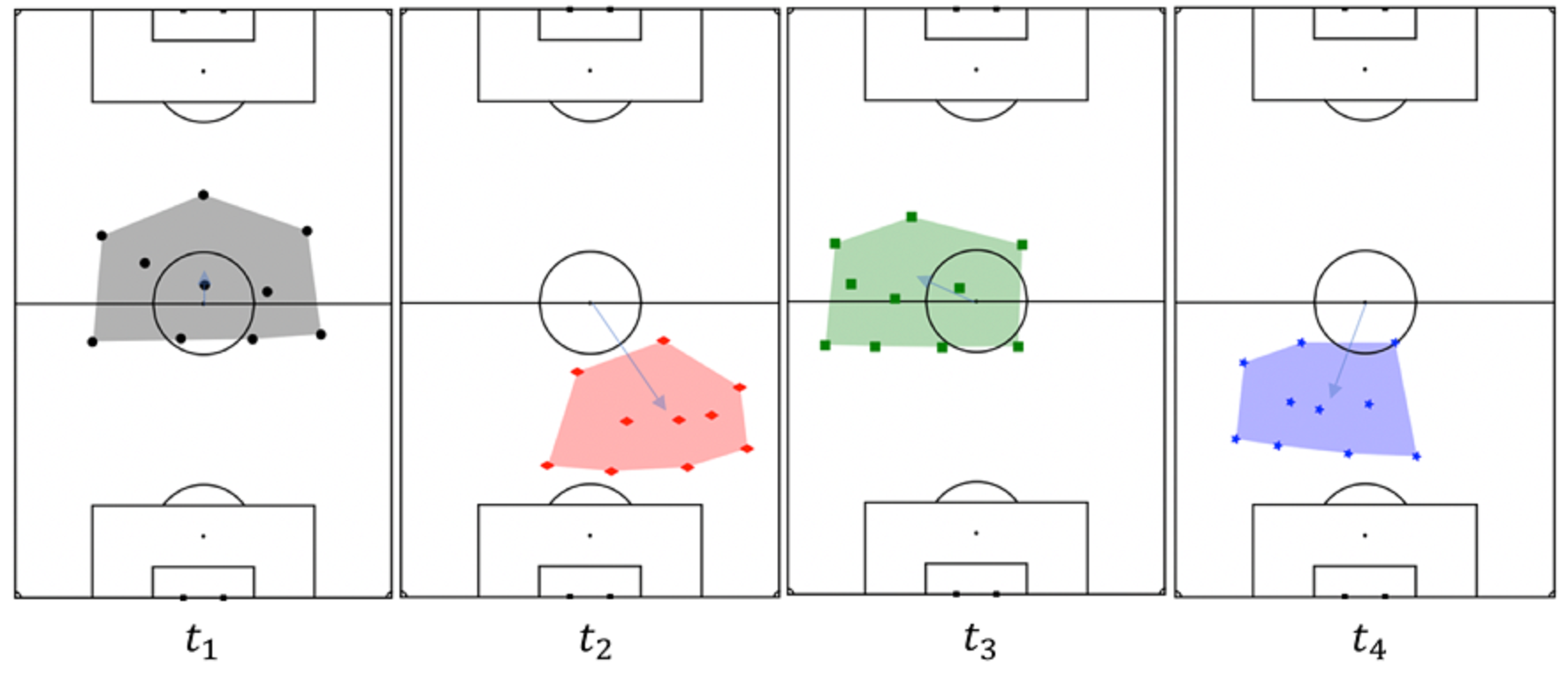
Figure 1: The positions of the outfield players of the defending team at four instants of time during a match. The shaded regions indicate the convex hull; the blue arrow indicates the centre of mass of the team relative to the centre of the pitch.
図1:試合中の4つの瞬間におけるディフェンス側の(GK以外の)選手の位置。 網掛け部分は凸包を示しています。 青い矢印は、ピッチの中心に対するチームの重心を示しています。
Formations are measured by calculating the vectors between each player and the rest of his teammates at successive instants during a match, averaging the vectors between each pair of players over a specified time interval to gain a clear measure of their designated relative positions. Defensive and offensive formation observations are measured separately by aggregating together consecutive possessions of the ball for each team into two-minute, non-contiguous time periods. We exclude possessions that last for less than five seconds from this process under the assumption that they are too short for either team to establish an offensive or defensive stance.Furthermore, if a substitution occurs – which may potentially be accompanied by a formation change – we end the window, retaining it in our analysis if it contains at least one minute of in-play data. Within each window we measure the formations of both the team in possession and their opponent. On average, we obtain ten defensive (i.e., out-of-possession) formation observations and ten offensive (in-possession) formation observations for each team during a match.
フォーメーションは、試合中の連続した瞬間に各プレイヤーと残りのチームメイトの間のベクトルを計算し、指定された時間間隔で各ペアのプレイヤー間のベクトルを平均して、指定された相対位置の明確な測定値を取得することによって測定されます。守備的および攻撃的なフォーメーションの観測値は、各チームのボールの連続したポゼッションを2分間の非連続時間に集約することによって個別に測定されます。どちらのチームにとっても攻撃的または守備的なスタンスを確立するには短すぎるという仮定の下で、このプロセスから5秒未満のポゼッションを除外します。さらに、フォーメーションの変更を伴う可能性のある(選手)交代が発生した場合、ウィンドウを終了し、少なくとも1分間のインプレイのデータが含まれている場合は分析で保持します。各ウィンドウ内で、ポゼッションしているチームと相手の両方のフォーメーションを測定します。平均して、試合中に各チームについて10の守備(つまり、ポゼッションしていない)フォーメーションの観測値と10の攻撃(ポゼッションしている)フォーメーションの観測値を取得します。
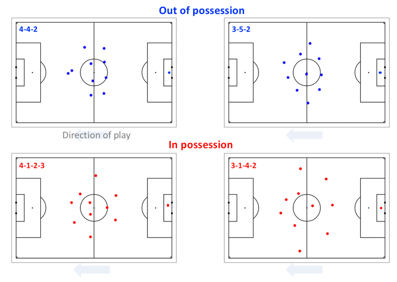
Figure 2 presents four examples of individual formation observations, each measured in a 2-minute aggregated possession window. The top two panels show defensive formation observations (out-of-possession);
図2は、個々のフォーメーションの観測値の4つの例を示しており,それぞれは、2分間の集約されたポゼッションウィンドウで測定されました。上の2つのパネルは、ディフェンシブなフォーメーションの観測値(ポゼッションしていない)を示しており、下の2つのパネルは、オフェンシブなフォーメーションの観測結果を示しています(ポゼッションしている)。
Figure 3 plots the full set of formation observations for one team during a single match.
It is clear that, when out of possession (upper plot), the team played with a 4-1-4-1 formation, with a single defensive central midfielder and a lone striker.
When in possession (lower plot), the outside midfielders advanced to form a front three and the full backs moved level with the defensive midfielder.
The right central midfielder played slightly deeper than the left central midfielder, introducing a small asymmetry to the team when attacking.
While the relative positions of the defensive players in the team are well constrained, the position of the offensive players – particularly the central striker – are much more broadly distributed, both in and out of possession.
More generally, the area encompassed by the outfield players (the convex hull) when attacking was twice the area encompassed when it was defending. The consistency of the observations indicates that the manager did not make a significant formation change during the match.
図3は、1回の試合中の1つのチームのフォーメーションの観測値の完全なセットをプロットしています。
ポゼッションしていない場合(上のプロット)、チームは4-1-4-1フォーメーションでプレーし、1人の守備的セントラルミッドフィルダーとワントップのストライカーでプレーしたことがわかります。
ポゼッションしているとき(下のプロット)、外側のミッドフィールダーが前進してフロントの3枚を形成し、バック全体が守備的ミッドフィールダーと同じレベルに移動しました。
右のセントラルミッドフィールダーは左のセントラルミッドフィールダーよりもわずかに深くプレーし、攻撃時に小さな非対称性をチームにもたらしました。
チーム内の守備側プレイヤーの相対的な位置は十分に制約されていますが、攻撃側プレイヤー、特に中央のストライカーの位置は、ポゼッションと非ポゼッションの両方ではるかに広く分散しています。
より一般的には、攻撃時に(GK以外の)選手が包囲する領域(凸包)は、守備時に包囲される領域の2倍でした。 観測値の一貫性は、監督が試合中に大きなフォーメーションの変更を行わなかったことを示しています。
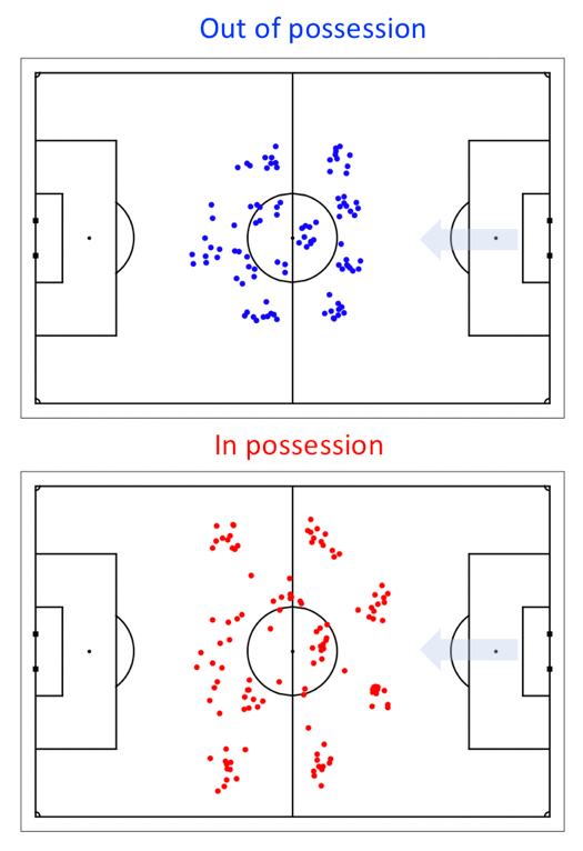
Figure 3: The full set of formation observations for one team throughout an entire match.The upper plot indicates the defensive formation observations, the lower plot indicates the offensive formation observations; in both cases, the team is shooting from right to left.The consistency of the observations indicates that the team did not undergo a significant formation change during the match.
図3:試合全体を通しての1つのチームのフォーメーションの観測値の完全なセットです。上のプロットはディフェンシブなフォーメーションの観測値を示し、下のプロットはオフェンシブなフォーメーションの観測値を示しています。 どちらの場合も、チームは右から左に攻撃しています。観測結果の一貫性は、試合中にチームが大きなフォーメーションの変更を受けなかったことを示しています。
Identifying unique formations
ユニーク(一意)なフォーメーションの特定
We applied the methodology described above to tracking data from a training sample of 100 matches, obtaining 3976 observations of offensive and defensive formations. In this section we describe the application of agglomerative hierarchical clustering to group similar observations to identify the set of unique formation types adopted by the teams during these matches.
上記の方法論を、100試合のトレーニングサンプルからのトラッキングデータに適用して、3976の攻撃的および守備的なフォーメーションの観測値を得ました。このセクションでは、類似の観測値をグループ化して、これらの試合中にチームによって採用された一意のフォーメーションタイプのセットを識別するための凝集型階層的クラスタリングの適用について説明します。
A key element of this process was to define a metric for quantifying the similarity of two formation observations. The technical details of how this is done are described in Appendix 1, but essentially we calculate the ‘cost’ of moving from one formation to another: the more different the formations, the higher the cost. Our method recognises that two formations might be identical in their shape (i.e. a 4-4-2), but one might be an expanded or compacted version of another. As we want to separate formations based on their shape, not their area, we rescale one of the formations during a comparison so that ‘compactness’ is no longer a discriminator.
このプロセスの重要な要素は、2つのフォーメーション観測値の類似性を定量化するためのメトリックを定義することでした。 これを行う方法の技術的な詳細はAppendix 1に記載されていますが、基本的に、あるフォーメーションから別のフォーメーションに移動する「コスト」を計算します。フォーメーションが異なるほど、コストが高くなります。私たちの方法では、2つのフォーメーションの形状が同一(4-4-2)である可能性がありますが、一方が他方のフォーメーションの拡張バージョンまたはコンパクトバージョンである可能性があることを認識しています。領域ではなく形状に基づいてフォーメーションを分離するため、比較中にフォーメーションの1つを再スケーリングして、「コンパクトさ」が差別化されないようにします。
We apply agglomerative hierarchical clustering to the formation observations measured from our training sample of matches. This identified 20 unique formation templates, or clusters, used by the teams in our training sample. The results are shown in Figure 4.
試合のトレーニングサンプルから測定されたフォーメーションの観測値に、凝集型階層的クラスタリングを適用します。結果を図4に示します。

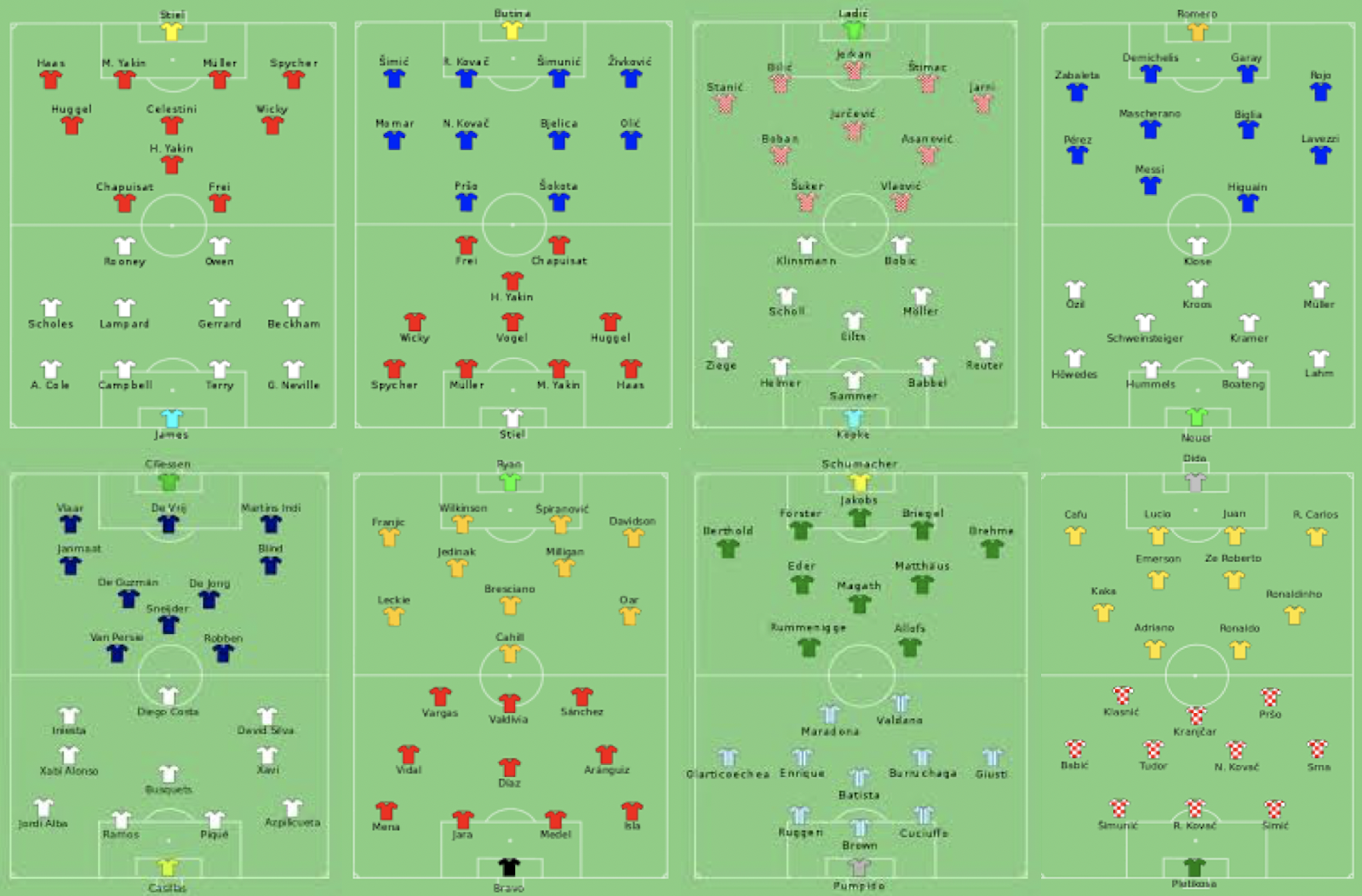
Figure 4: The 20 unique formation clusters identified using hierarchical clustering based on a training sample of formations measured in 100 professional matches. Teams are orientated to shoot from right to left, and formations are translated to align their centre of mass with the centre of the pitch. Ellipses indicate the 1-sigma region (68% confidence interval) for the positions of each player, measured over the individual observations in each cluster.The text in the bottom left of each panel indicates the proportion of offensive and defensive formation observations in the cluster (also indicated by the green and red bars).
図4:100のプロの試合で測定されたフォーメーションのトレーニングサンプルに基づく階層的クラスタリングを使用して特定された20のユニークなフォーメーションクラスター。チームは右から左に攻撃するように方向付けられており、フォーメーションは重心をピッチの中心に合わせるために変換されています。
楕円は、各クラスターの個々の観測値で測定された、各プレーヤーの位置の1シグマ区間(68%の信頼区間)を示します。各パネルの左下のテキストは、クラスター内のオフェンシブおよびディフェンシブなフォーメーション観測値の割合を示しています(緑と赤のバーでも示されています)。
There is a clear ordering to the clusters that highlights the difference between defensive and offensive formations – a distinction lost in previous analyses of formations in football. The top row in Figure 4 contains formation clusters with five defenders and variations in the number of midfielders and forwards; these clusters predominantly consist of defensive formation observations.The following two rows indicate variants of a back four: cluster 6 is clearly a midfield diamond, clusters 9 and 10 are variants of a 4-3-3 formation, cluster 11 is a 4-1-4-1 and cluster 12 is a 4-4-2. The clusters in these rows contain a mix of attacking and defensive formation observations. For instance, cluster 9 predominantly consists of defensive formation observations, while cluster 10 is mostly made up of offensive observations.
クラスターの順序は明確で、ディフェンシブとオフェンシブなフォーメーションの違いを強調しています。これは、サッカーのフォーメーションの以前の分析では失われた区別です。図4の一番上の行には、5人のディフェンダーと、ミッドフィルダーとフォワードの数のバリエーションを持つフォーメーションクラスターが含まれています。 これらのクラスターは、主にディフェンシブなフォーメーションの観測値で構成されています。次の2行は、4バックのバリエーションを示しています。Cluster6は明らかにダイアモンド型の中盤、Cluster9と10は4-3-3フォーメーションのバリエーション、Cluster11は4-1-4-1、Cluster12は 4-4-2です。これらの行のクラスターには、オフェンスとディフェンスのフォーメーションの観測値が混在しています。たとえば、Cluster9は主にディフェンシブなフォーメーションの観測値で構成され、Cluster10はほとんどがオフェンシブな観測値で構成されています。
The fourth and fifth rows contain clusters that almost entirely consist of offensive formation observations. The fourth row contains variants of the 3-4-3 and 3-5-2 formations, although the standard nomenclature is a crude description of these formations. The fifth row shows clusters that have essentially just two defensive players – in all four cases the full-back positions have advanced significantly.
4行目と5行目には、ほぼ完全にオフェンシブなフォーメーションの観測値で構成されるクラスターが含まれています。4番目の行には、3-4-3および3-5-2フォーメーションのバリエーションが含まれていますが、標準の命名法はこれらのフォーメーションの大まかな説明です。5番目の行は、基本的にディフェンスプレイヤーが2人だけのクラスターを示しています。4つすべてのケースで、フルバックのポジションが大幅に進歩しています。
Overall, it is clear that the hierarchical clustering has efficiently separated observations of defensive and offensive formations, even though it could not use the differences in their size, or area encompassed, as a discriminator (because of our application of the scaling factor, k as described in Appendix 1).
全体として、階層的クラスタリングは、サイズまたは囲んだ領域の違いを識別器として使用できなかったとしても、ディフェンス形成とオフェンス形成の観察を効率的に分離したことは明らかです(Appendix 1で説明したように、スケーリング係数kの適用のため)。
Formation classification
フォーメーションの分類
The final step of our methodology is a Bayesian model selection algorithm to estimate the probability that a newly observed formation belongs to each of the 20 formation clusters shown in Figure 4; the mathematical details are given in Appendix 2.Identifying the maximum probability cluster for each formation observation enables us to classify formation observations throughout a match to dynamically detect tactical changes.
私たちの方法論の最後のステップは、新たに観測されたフォーメーションが図4に示す20のフォーメーションクラスターのそれぞれに属する確率を推定するベイズモデル選択アルゴリズムです;数学的な詳細はAppendix 2に記載されています。各フォーメーション観測値の最大確率のクラスターを特定することで、試合全体でフォーメーションの観測値を分類し、戦術的な変化を動的に検出できます。
Results and analysis
結果と分析
We first investigated transitions between defence and offence by identifying the defensive and offensive formation clusters that are most frequently paired together by the teams in our dataset. In Figure 5 we plot an example of these pairings using a Sankey diagram. The left-hand side of the diagram corresponds to defensive formation clusters, while the right-hand side corresponds to offensive formation clusters. The links between them indicate the formations that were typically employed together as teams gained and lost possession.
最初に、データセットの中のチームで最も頻繁にペアリングされるディフェンスおよびオフェンスフォーメーションのクラスターを特定することにより、ディフェンスとオフェンスの間の変位を調べました。図5では、サンキー・ダイアグラムを使用してこれらのペアリングの例をプロットしています。図の左側はディフェンスフォーメーションクラスターに対応し、右側はオフェンスフォーメーションクラスターに対応します。
それらの間のリンクは、チームがポゼションを獲得したり失ったりしたときに通常一緒に採用されたフォーメーションを示しています。

Figure 5: Two examples of the typical pairings between defensive and offensive formations.
The blue formations indicate that teams playing with a defensive formation drawn from cluster 2 (see Figure 4) transition to an offensive formation drawn from cluster 16. The red example indicates that teams that play with defensive formation 9 transition to either offensive formations 10 or 18. All teams are orientated to shoot from right to left.
図5:ディフェンスフォーメーションとオフェンスフォーメーションの典型的な組み合わせの2つの例。
青いフォーメーションは、Cluster2(図4を参照)から引き出されたディフェンスフォーメーションでプレイしているチームが、Cluster16から引き出されたオフェンスフォーメーションへ変位することを示しています。
赤色の例は、ディフェンスフォーメーション9でプレイするチームが、オフェンスフォーメーション10または18へ変位することを示しています。すべてのチームは、右から左に攻撃する向きになっています。
The example highlighted in blue indicates that teams in our sample that defended using cluster 2 (as defined in Figure 4) transitioned to cluster 16 when in possession of the ball. The connection between the two formations is clear: the outside defenders, or wingbacks, advance when the team gains possession and the two outside midfielders tuck in behind the two forwards.
青色で強調表示されている例は、ボールをポゼションしているときにCluster2(図4で定義)を使用してディフェンスしたサンプルのチームが、Cluster16へ変位したことを示しています。2つのフォーメーションの関係は明らかです。外側のディフェンダーまたはウィングバックは、チームがポゼションを獲得し、2人の外側のミッドフィールダーが2人のフォワードの後ろに押し込まれると前進します。
The second example, highlighted in red, demonstrates that teams using cluster 9 (a 4-3-3) when defending would transition into either cluster 10 or cluster 18 when attacking – two formations that are quite different. In cluster 10, the outside forwards have pushed wide and the full-backs have advanced, whereas in cluster 18 the front three remain narrow with the full-backs advancing further up the field to provide width.
赤で強調表示されている2番目の例は、ディフェンス時にCluster9(4-3-3)を使用しているチームが、オフェンス時にCluster10またはCluster18に変位することを示しています。Cluster10では、外側のフォワードが広く押し出され、フルバックが進みましたが、一方Cluster18では、フロントの3枚が狭いままで、フルバックがフィールドをさらに進んで幅を提供します。
There are two main conclusions to draw from these examples. First, the defensive and offensive formation pairings are consistent: it is clear how each player’s defensive and offensive roles are related. This provides an important validation of our methodology. Second, it demonstrates that some defensive configurations provide more flexibility in terms of different attacking options than others.
これらの例から引き出される主な結論は2つあります。一つ目は、ディフェンスとオフェンスのフォーメーションの組み合わせは一貫しています。各プレイヤーのディフェンスとオフェンスの役割がどのように関連しているかは明らかです。これは、方法論の重要な検証を提供します。二つ目は、いくつかのディフェンス構成は、他の構成よりもさまざまなオフェンスオプションに関して柔軟性が高いことを示しています。
Strategic summaries and changes in formations
戦略の概要とフォーメーションの変更
Dynamic measurement and classification of formations enable us to produce strategic summaries of matches that communicates the defensive and offensive configurations of each team and detects when major tactical changes occurred.
フォーメーションの動的な測定と分類は、各チームの守備的および攻撃的な構成を伝え、主要な戦術変更の発生時にはそれを検出する、試合の戦略的要約を作成できます。
Figure 6 charts the defensive and offensive formations during a match between two teams – labelled the Red team and the Blue team – throughout the course of a match. The circles indicate the offensive formation observations of each team, classified according to the clusters shown in Figure 4; the diamonds indicate the defensive formations. Goals are indicated by a vertical dashed line at the top of the plot; substitutions are indicated by a vertical dashed line along the bottom of the plot.
図6は、試合中の2つのチーム(赤チームと青チーム)の試合中の守備と攻撃のフォーメーションを示しています。丸(◯)は、図4に示すクラスターに従って分類された各チームの攻撃フォーメーションの観察結果を示しています;ひし形(◇)は守備的なフォーメーションを示しています。 ゴールは、プロットの上部に縦の破線で示されます;(選手)交代は、プロットの下部に沿って垂直の破線で示されます。
In this match, the Red team were losing 1-0 at half time.The chart indicates that the manager made a substitution and a significant change in formation, switching from a 3-4-3 formation (clusters 3 and 15 in defensive and attack, respectively) to a 4-3-3 (clusters 9 and 10). They scored shortly after half time, but ultimately lost the match 2-1.
この試合では、赤チームはハーフタイム時には1-0で負けていました。このグラフは、監督が(選手)交代とフォーメーションの大幅な変更を行い、3-4-3フォーメーション(それぞれ守備と攻撃のCluster3と15)から4-3-3(Cluster9と10)に切り替えたことを示しています。ハーフタイム後すぐに得点しましたが、最終的には2-1で敗れました。
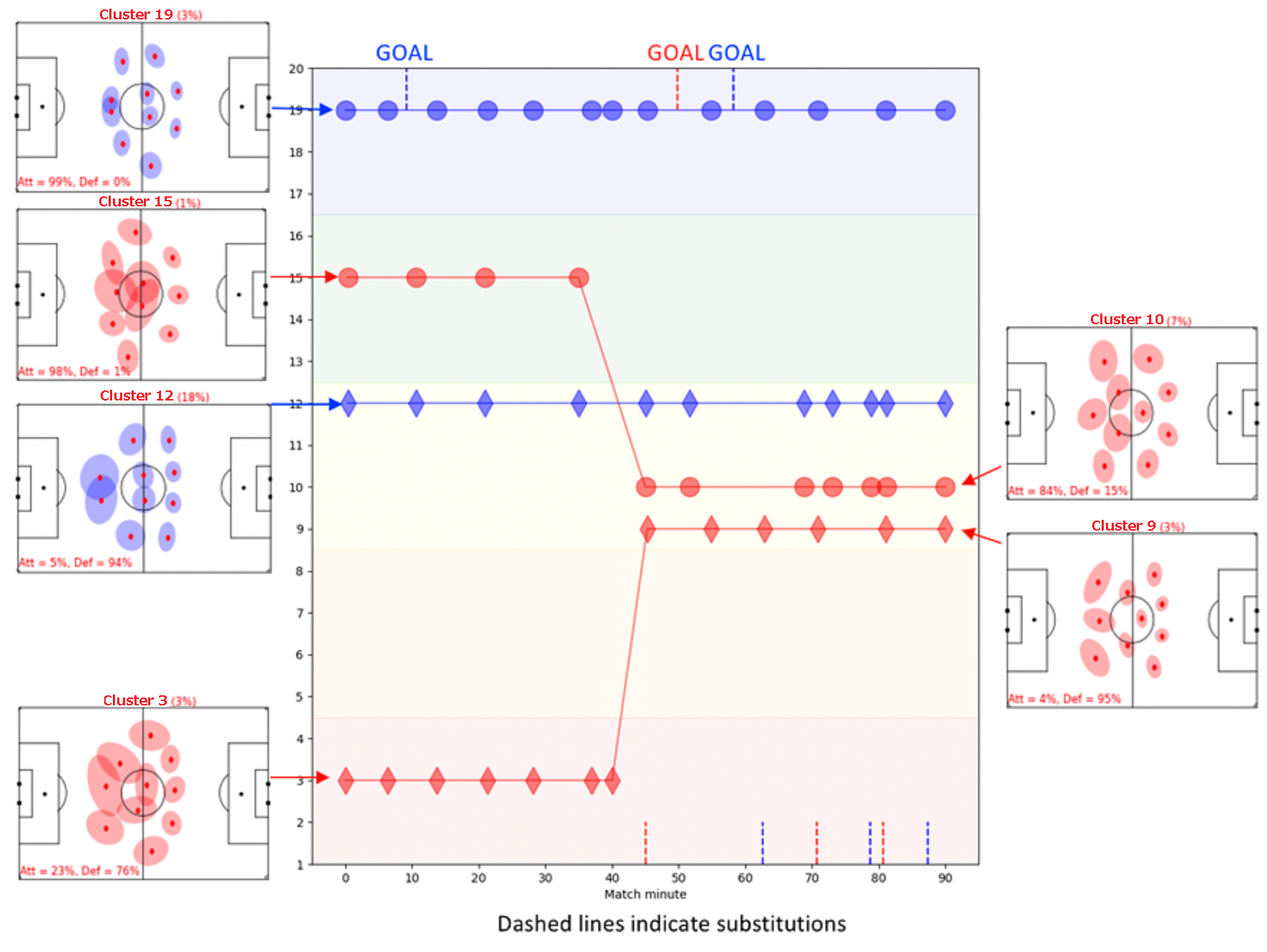
Figure 6: Strategic summary of a match between the Red and Blue teams. Diamonds indicate defensive formations; circles indicate offensive formations. Y-axis labels correspond to the cluster numbers in Figure 4.
図6:赤チームと青チームの試合の戦略的概要。ひし形(◇)は守備的なフォーメーションを示します。 丸(◯)は攻撃的なフォーメーションを示します。 Y軸のラベルは、図4のクラスター番号に対応しています。
Automated detection of formation changes, combined with event data, enable us to investigate why certain tactical changes were made and evaluate the impact they had on the outcome of a match.
Figure 7 shows a simple example (a different match that depicted in Figure 6: the Red team is the same, but they are playing a different Blue team). The right-hand panels of the plot indicate the defensive formation observations of the Red team in the first and second half. The left-hand panels show pass and shot maps of the opposing team (shooting from left to right); arrows indicate individual passes and dots denote shots, with the symbol size indicating the quality of the opportunity.
イベントデータと組み合わされたフォーメーション変更の自動検出により、特定の戦術的な変更が行われた理由を調べ、試合の結果に与える影響を評価できます。図7は、単純な例を示しています(図6に示されているものとは異なる試合:赤チームは同じですが、彼らは異なる青チームとプレイしています)。プロットの右側のパネルは、前半と後半の赤チームのディフェンスフォーメーションの観測値を示しています。左側のパネルには、相手チームのパスとシュートのマップが表示されます(左から右に攻撃)。 矢印は個々のパスを示し、ドットはシュートを示し、シンボルサイズはチャンスの質を示します。
In the first half, the Red team played with a 4-3-3 in defence. The pass map of the Blue team indicates that they tended to attack down the flanks in the first half, creating high-quality chances from crosses, particularly from the right wing. At half time the Red team switched to a 5-man defence, with the wing-backs marking the opposing wingers. As the pass map for the second half indicates, the change in formation appears to have been effective in preventing the Blue team creating chances from their right side, with the focus of their passing switching more towards the centre and left of the pitch.
前半、赤チームはディフェンス時には4-3-3でプレーしました。青チームのパスマップは、彼らが前半にサイドから攻撃する傾向があり、特に右からのクロスから高品質のチャンスを作り出したことを示しています。
ハーフタイムに赤チームは5枚のディフェンスに切り替え、ウィングバックが相手のウィンガーをマークしました。後半のパスマップが示すように、フォーメーションの変更は、青チームが右側からチャンスを生み出すのを防ぐのに効果的であるように思われ、パスの焦点はピッチの中央と左側に向かってより多く切り替わっています。
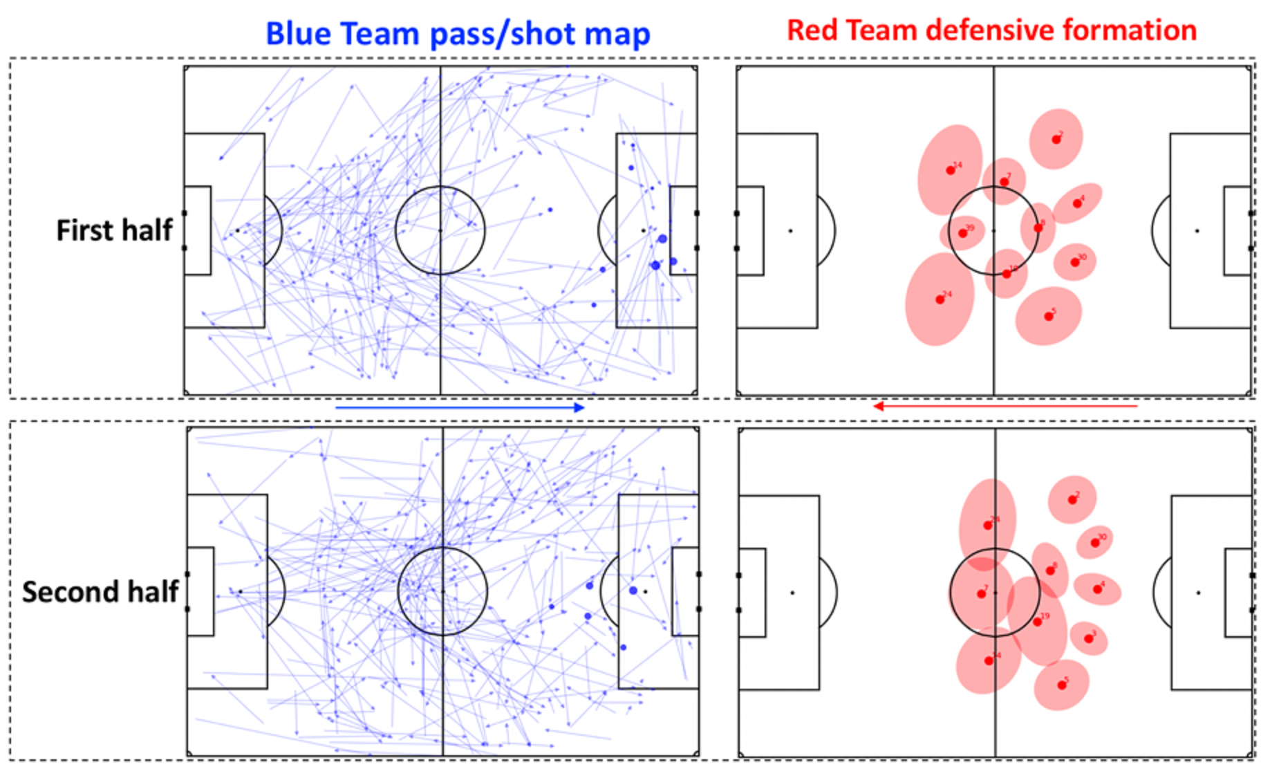
Figure 7: Right hand plots: observations of the defensive formation of the Red team (playing from right to left) before and after half time in a match against the Blue team.Left hand plots: passes (arrows) and shots (circles) of the blue team (playing from left to right) in the first and second half of the match. The sizes of the circles indicate the quality of the shooting opportunity. Note that the match depicted is different to the match shown in Figure 6.
図7:右側のプロット:青チームとの試合でハーフタイムの前後に赤チーム(右から左へプレイ)の守備フォーメーションの観測値。左側のプロット:試合の前半と後半の青チーム(左から右にプレー)のパス(矢印)とシュート(円)。円のサイズは、攻撃チャンスの質を示しています。 示されている一致は、図6に示されている一致とは異なることに注意してください。
Practical applications
実用的な応用
Our analysis is a step towards the use of tracking data to infer and evaluate team strategy in football. The methodology outlined above enables teams to study how an opposing manager habitually responds to specific match situations. For instance, the manager of the Red Team in Figure 6 made similar formation changes at (or near to) half time in over a quarter of their matches in our dataset, switching between a small subset of formations based on the quality of the opposition and the state of the match.Our methodology can be used to anticipate and exploit opposition tactical changes.
私たちの分析は、サッカーのチーム戦略を推測および評価するためのトラキングデータの使用に向けた一歩です。上記で概説した方法論により、チームは特定の試合の状況に対して相手の監督が習慣的にどのように対応するかを研究できます。たとえば、図6の赤チームの監督は、データセットでの試合の4分の1以上で、ハーフタイム(またはそれに近い)時点で、相手チームの質と試合の状態に基づいてフォーメーションの小さなサブセットを切り替えながら、同様のフォーメーションの変更を行いました。私たちの方法論は、相手チームの戦術的変化を予測して活用するために使用できます。
Second, it enables us to study in detail the factors that cause the defensive formation of a team to become disrupted and investigate how this relates to chance creation.Combining formation classification with pitch control surfaces [11,12,13] enables us to identify potential defensive weaknesses of specific formations and determine how teams might exploit them.
第二に、チームの守備的なフォーメーションを混乱させる要因を詳細に研究し、これがチャンスの創造にどのように関係するかを調査することを可能にします。フォーメーション分類とピッチコントロールサーフェス[11,12,13]を組み合わせることで、特定のフォーメーションの潜在的な防御上の弱点を特定し、チームがそれらを活用する方法を決定できます。
Finally, our methodology can be extended to consider formations in more specific phases of possessions, such as transition, establishing possession, progression and chance creation, and to incorporate player velocity information to identify and understand marking systems and the operation of a high press.
最後に、方法論を拡張して、移行、ポゼションの確立、進行、チャンスの作成など、ポゼションのより具体的な段階でのフォーメーションを検討し、プレイヤーの速度情報を組み込んで、マーキングシステムとハイプレスの操作を識別して理解することができます。
Appendix 1: Formation Similarity
Appendix 1: フォーメーションの類似性
In our method, a formation observation is effectively a set of 10 bivariate normal distributions – one for each outfield player – in which the mean of each distribution is the position of a player in the formation (remembering that the formations are translated so that the centres of mass coincide), and the covariance matrix is an estimation of how far the player deviated from his position during the two minute possession window in which the formation was measured.
私たちの方法では、フォーメーションの観測値は事実上10個の2変量正規分布のセットです(GK以外の各プレーヤーに1つずつ)。各分布の平均はフォーメーション内のプレーヤーの位置です(重心が一致するようにフォーメーションが変換されることを思い出してください)、そして共分散行列は、フォーメーションが測定された2分間のポゼションウィンドウの中でプレイヤーが自分の位置からどれだけ逸脱したかの推定値です。
We utilize the Wasserstein distance [5] to quantify the similarity of two formation observations. In the simple case of two bivariate normal distributions、μ1=N(m1,C1) and μ2=N(m2,C2), where m is the mean and C is the covariance matrix, the square of the Wasserstein distance is given by [6]:
Wasserstein距離[5]を使用して、2つのフォーメーションの観測値の類似性を定量化します。 2つの2変量正規分布の単純な場合μ1=N(m1,C1) そして μ2=N(m2,C2)、ここで、mは平均、Cは共分散行列です。Wasserstein距離の2乗は[6]で与えられます:
$$\Large{W(\mu_1,\mu_2)^2 = \|m_1 – m_2\|^2 + trace(C_1 + C_2 – 2(C_2^\frac{1}{2}C_1C_2^\frac{1}{2})^\frac{1}{2})}$$
In the case of point particles the Wasserstein distance is simply the square root of the L2 norm of the difference between the means. More generally, the Wasserstein metric is a solution to the optimal transport problem [7], i.e., an estimate of the cost of moving from one distribution to another.
点粒子の場合、Wasserstein距離は、単に平均間の差のL2ノルムの平方根です。 より一般的には、Wasserstein計量は、最適な輸送問題[7]の解決策です。つまり、ある分布から別の分布に移動するコストの推定値です。
The second step of our algorithm is to find a pairing of the players in the two formation observations that minimizes the square of the sum of the Wasserstein distances, i.e.
アルゴリズムの2番目のステップは、2つのフォーメーションの観測値で、Wasserstein距離の合計の2乗を最小化するプレイヤーのペアを見つけることです。
$$\Large{W^2_{total} = min \sum_i\sum_jD_{ij}X_{ij}}$$
where Dij is the cost (square of Wasserstein distance) of matching player i in formation 1 to player j in formation 2, and Xij is a player-player allocation matrix, in which each element is equal to 1 if player i is matched to player j, and zero otherwise. Each row and column in Xij must therefore uniquely consist of nine 0s and a single 1. We use the Kuhn-Munkres algorithm [8,9] to find the Xij that minimises the total cost.
ここで、Dijは、フォーメーション1のプレーヤーiをフォーメーション2のプレーヤーjに一致させるコスト(Wasserstein距離の2乗)です。Xijは、プレーヤー-プレーヤー割り当てマトリックスです。
プレーヤーiがプレーヤーjに一致する場合、各要素は1 、それ以外の場合はゼロ。
したがって、Xijの各行と列は、9個の0と1個の1で一意に構成する必要があります。Kuhn-Munkresアルゴリズム[8,9]を使用して、総コストを最小化するXijを見つけます。
We make one further extension to our metric for team similarity.
Two formation observations may be identical in terms of their shape (e.g. a traditional 4-4-2), but one may be a more compact or expanded incidence of the other.
As we aim to identify distinct formation shapes, we introduce a variable scaling factor, k , that expands or contracts a formation around its centre of mass (scaling the player covariances accordingly).
When comparing two formation observations, we search for the value of k that minimises the Wasserstein distance between them.
チームの類似性に関するメトリックをさらに拡張します。
2つのフォーメーションの観測結果は、形状に関しては同じ場合があります(たとえば、従来の4-4-2)が、一方が他方をよりコンパクトにしたもの、または拡大されたものである可能性があります。
異なるフォーメーションの形状を識別することを目的として、その重心の周りでフォーメーションを拡大または縮小する可変のスケーリング係数kを導入します(それに応じてプレーヤーの共分散をスケーリングします)。
2つのフォーメーションの観測値を比較するとき、それらの間のWasserstein距離を最小にするkの値を検索します。
Appendix 2: Formation Classification Algorithm
Appendix 2: フォーメーション分類アルゴリズム
The Bayesian model selection algorithm for estimating the probability that a newly observed formation belongs to each of the 20 formation clusters shown in Figure 4 is calculated as
図4に示す20のフォーメーションクラスターのそれぞれに新しく観測されたフォーメーションが属する確率を推定するためのベイズモデル選択アルゴリズムは、以下の式で計算されます。
$$\Large{p(o|C)\sim \underset{k}{\mathrm{argmax}} \displaystyle\prod_{p=1}^{10} \displaystyle\int {\rm p}(y| kμ_{p,C}, k^2 \Sigma_{p,C}){\rm p}(y|μ_{p,o}, \Sigma_{p,o} ){\rm d}y\;}$$
where μp,C and Σp,C are the position and covariance matrix for role p in cluster C , μp,o and Σp,o are the position and covariance matrix for player p in the formation observation o , k is the scaling factor described in Appendix 1, and the integral is performed over the surface area of the pitch.
To assign each player in a formation observation to a specific role in a cluster, we solve the player-role allocation problem using the Kuhn-Munkres algorithm, also described in Appendix 1.
ここで、μp、CとΣp、CはクラスターCのrole pの位置と共分散行列、μp、oとΣp、oはフォーメーションの観測値 oのplayer pの位置と共分散行列、kは Appendix 1にあるスケールファクター、そして積分はピッチの全面にわたって実行されます。
フォーメーションの観測値の各playerをクラスター内の特定のroleに割り当てるには、Kunn-Munkresアルゴリズム(Appendix 1でも説明)を使用して、player-role の割り当て問題を解きます。
Appendix 3
data driven
データ駆動
agglomerative hierarchical clustering
凝集型階層的クラスタリング
Bayesian model selection
ベイジアンモデル選択
window
ウィンドウ
すみません、うまく訳せません。対象領域を特定する矩形枠….くらいのイメージ?
探索領域のほうがピンとくるかな。
画像認識の学習でsliding windowという手法が使われますが、そういう感じかな?
1-sigma region
1シグマ区間
Sankey diagram
サンキー・ダイアグラム
コードで使ってみたい方参照:riverplot
Wasserstein distance、L2 norm
Wasserstein(ワッサースタイン)距離、L2 ノルム
機械学習ではいろいろな「距離」の概念が使われます。Wasserstein 距離はそのうちの1つです。
L2ノルムは、連続的な分布における二乗誤差の和のこと(高校までの「普通の意味での長さ」、ユークリッドノルムとも言う)。
この論文で使われている式については[5]参照、arXivはここ
Kuhn-Munkres algorithm
Kuhn-Munkres アルゴリズム
Player,Role
すみません、うまく訳せません。もしかしたら、player – 選手、role – 役割(プレイ)でいいのかもしれませんが。
bivariate normal distribution
2変量正規分布
2次元正規分布
References
その他の参考文献
トラッキングデータを用いたサッカーの試合における戦況変化の抽出
サッカーのトラッキングデータからの守備戦術プレーの達成度評価
なでしこの猶本選手や安藤選手(元?)が論文の共同執筆にいますなぁ….ふむふむ(筑波だからね)
サッカートラッキングデータを用いた機械学習に基づくプレー認識手法の提案
以下は現在paperを探しています
優秀賞「ガンバ大阪がリーグ優勝するためにーシュート数増加のための要因分析ー」
このフォーメーションの変位はピッチ上で選手が最も敏感に察知するところじゃないでしょうか?
それに対応できること…監督がフォーメーションを選んだ意味の理解力、戦術理解度が個々の選手に求められます。
サポーターも察知したいところ、ゴール裏はアホばっかりという評判を覆したいものです(アホはサポにとって重要な資質ではあるんですが)
…….(^^)。
ところで….
いつかは無くなるかも知れないけど、こんな記事もありました。
『戦術の教科書』(ジョナサン・ウィルソン、田邊雅之著/2017年刊)から、一部を抜粋して全3回で公開
グアルディオラVSモウリーニョ。対極に位置する2つのサッカーはどのようにして生まれたのか【戦術の教科書(1)】
ボール支配率の時代は終わった。根底から揺らいだボゼッションサッカーの系譜【戦術の教科書(2)】
ユルゲン・クロップを生み出したグアルディオラの存在。混沌と化す新たな戦術の時代【戦術の教科書(3)】
Next
これも面白そうな記事です。
AUTOMATED TRACKING OF BODY POSITIONING USING MATCH FOOTAGE
サッカー選手が次のプレイの準備のために体の面を作っておくことに関連したもののようです。
ゲーム中の選手の体の向きを3つの方法で推定・検出してみるというものです。
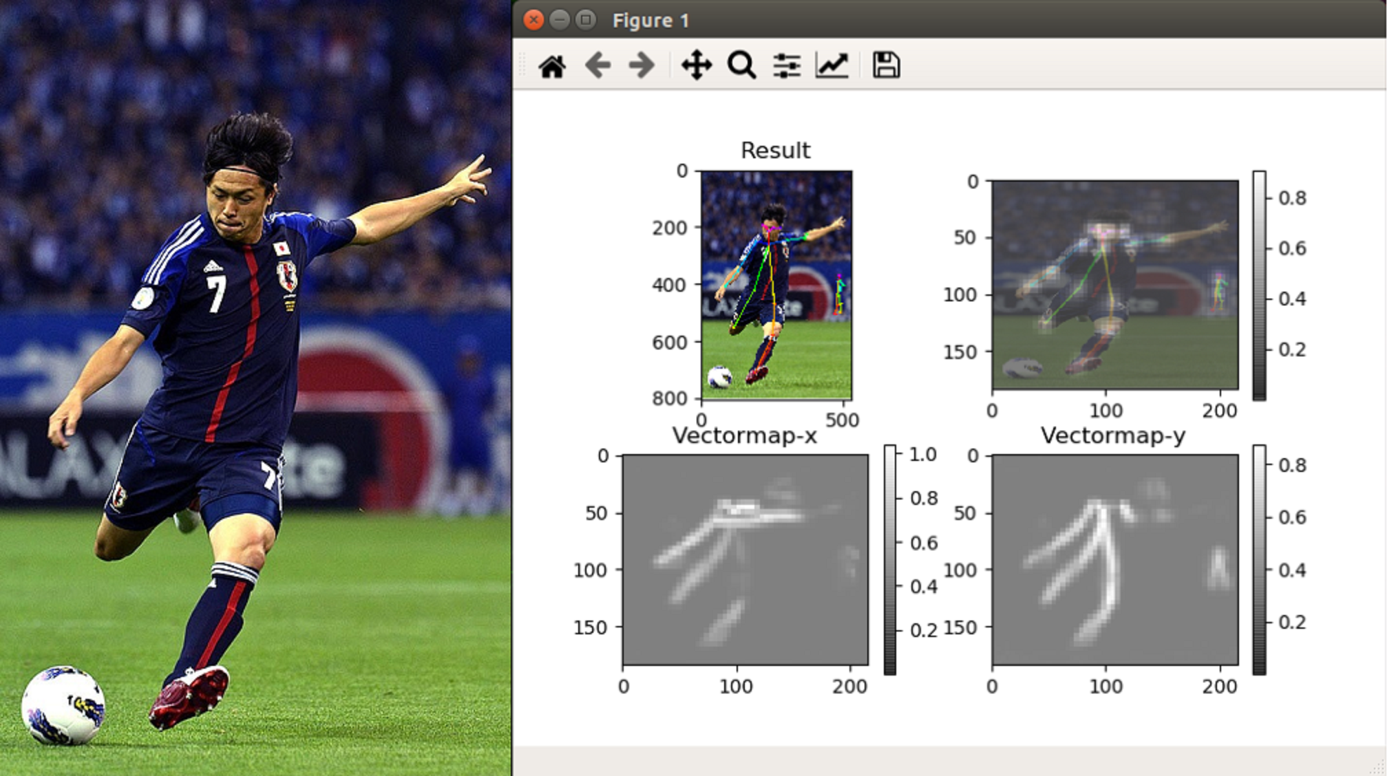
OpenPoseが使われています。これを使えば姿勢検出もできます。
ちなみに、ヤットさんの姿勢検出してみました、こんな感じ。
右端中央で検出されているのは、ただのボールボーイです(^^)。
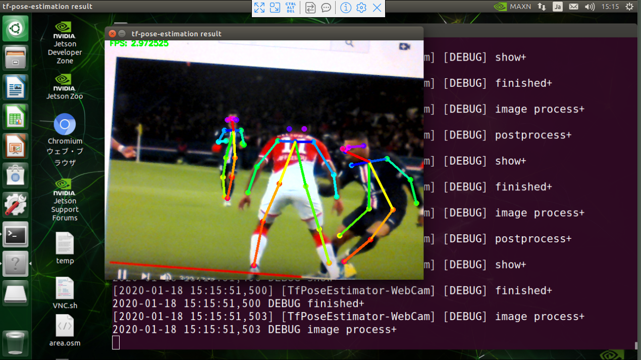
WebCamを使ってYoutube動画で検出してみる場合(FPSは3くらい出てます)
右がムバッペ(PSG)、対峙するモナコのディフェンダーという構図、ムバッペにPAに侵入され、この後ディフェンダーは抜かれて、一瞬出した左脚が引っかかってPK取られてます(TT;
Leave a Reply